Alekseev-Gröbner formula

Let $y(x)$ be the solution to the system of differential equation

with initial condition $y(x_0)=y_0$, and let ${\varphi }^{t_0,t_1}$ denote its flow, starting at time $t_0$ and ending at time $T$. Let $z(x)$ be the solution to the perturbed equation

where $({\varphi }^{s,x}{)}_{\ast }$ represents the pushforward (Jacobian) of the unperturbed flow evaluated along the perturbed trajectory $z(s)$ (see flow of a non-autonomous vector field).

Proof via Geometric Construction

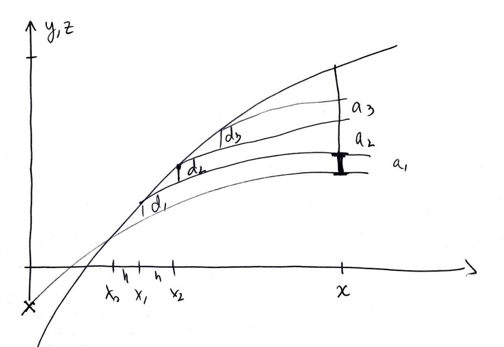
Partition the time interval $[x_0,x]$ into discrete steps of width $h$, yielding points $x_i=x_0+ih$.
At each step, the perturbation vector field $g$ creates a local, instantaneous deviation $d_i$ from the unperturbed trajectory. For the first step at $x_0$, this deviation is:

To determine how this local error impacts the solution at the final time $x$, it is transported forward along the unperturbed flow. By linearizing the flow operator, the propagated deviation $a_1$ at time $x$ is obtained by applying the pushforward $({\varphi }^{x_0,x}{)}_{\ast }$ to the initial deviation:

This process applies sequentially at every arbitrary time step $x_i$. For example, at $x_1$, the local deviation is evaluated along the perturbed trajectory $z(x_1)$:

The deviation $d_2$ is then propagated forward from $x_1$ to $x$:

In general, the propagated deviation for step $i$ (originating at $x_{i-1}$) is:

The total accumulated error between the perturbed trajectory $z(x)$ and the unperturbed trajectory $y(x)$ is approximated by summing all these independently propagated local deviations:

Substituting the general expression for $a_i$ yields the Riemann sum:

Taking the continuous limit as the step size $h\to 0$,