Cartan-Kähler theory

Integral elements and polar spaces

Recall that an integral element of an exterior differential system $(E, Ω)$ at $x \in M$ is a subspace $E \subset T_{x} M$ such that $ϕ |_{E} = 0$ for every $ϕ \in E$ . Integral elements are the candidates for tangent spaces to integral manifolds.

Definition (polar space). Let $E \subset T_{x} M$ be a $k$ -dimensional integral element of an EDS $(E, Ω)$ . Its polar space $H (E)$ is the set of vectors $v \in T_{x} M$ such that the subspace $E + ⟨ v ⟩$ is also an integral element. Equivalently,

H (E) := {v \in T_{x} M : ϕ |_{E + ⟨ v ⟩} = 0, for all ϕ \in E} .

The polar space is a linear subspace of $T_{x} M$ defined by the linear equations obtained by plugging $v$ into the forms of $E$ (filled with the vectors of $E$ ).

Basic properties.

$E \subseteq H (E)$ — every vector already in $E$ trivially extends $E$ to a larger integral element.
$\dim H (E) \geq \dim E$ always, with equality iff $E$ is maximal (no larger integral element contains it).
If $E$ is an integral element, any $(k + 1)$ -dimensional integral element $E^{+}$ that contains $E$ must satisfy $E^{+} \subseteq H (E)$ .

The flag of polar spaces

Let $(0) = E_{0} ⊊ E_{1} ⊊ \dots ⊊ E_{n}$ be a flag of integral elements, with $\dim E_{i} = i$ . (In practice, $E_{n}$ is an $n$ -dimensional integral element, the tangent space to an $n$ -dimensional integral manifold.) The polar spaces satisfy a descending flag:

T_{p} M \supseteq H (E_{0}) \supseteq H (E_{1}) \supseteq \dots \supseteq H (E_{n - 1}) \supseteq H (E_{n}) \supseteq E_{n} .

Why descending? The larger the integral element $E$ , the more vectors satisfy the linear conditions that define $H (E)$ — the polar equations become more restrictive. Thus $H (E_{i})$ shrinks as $i$ grows.

Cartan characters

For a flag $E_{0} \subset \dots \subset E_{n}$ in general position (a regular flag), define the integers

s_{j} := \dim H (E_{j - 1}) - \dim H (E_{j}), j = 1, \dots, n,

called the Cartan characters. We have:

$s_{0}$ : The number of restrictions imposed by the 1-forms in your ideal to find the initial polar space $H (E_{0})$ .
$s_{1}$ : The number of new restrictions imposed by the 2-forms (evaluated on a generic vector $v_{1} \in E_{1}$ ) to find $H (E_{1})$ .
$s_{2}$ : The number of new restrictions imposed by the forms to find $H (E_{2})$ .
...
$s_{k}$ : The number of new restrictions added when extending a generic $(k - 1)$ -dimensional integral element to a $k$ -dimensional one.

The Cartan procedure

See @bryant1999nine page 25.

Fase 1: extending a point into a curve

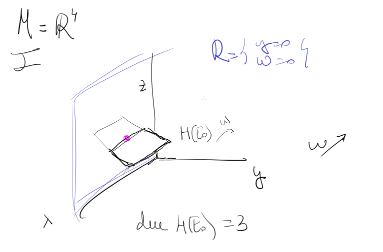
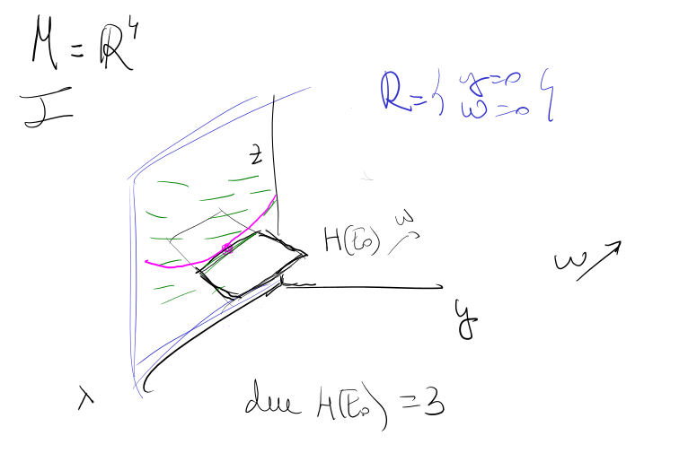
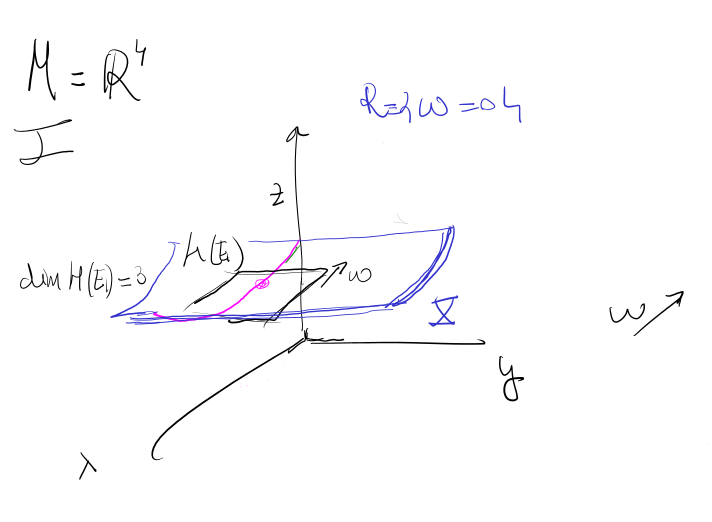
Consider an ambient manifold $M$ as a 4-dimensional space ( $\dim M = 4$ ), and a given differentially closed ideal $I$ . We start with a 0-dimensional manifold $P = {p_{0}}$ to be extended to a 1D integral manifold $X$ . We will assume $r = 2$ (see @bryant1999nine). That is, $d i m H (E_{0}) = 3$ .

Step 1: Where is the freedom of choice?

We have massive freedom to decide how to extend our point into a curve. Bryant handles this freedom immediately by asking us to choose a generic codimension- $r$ submanifold $R$ that contains our point $P$ . So, $R$ is an arbitrary 2D surface passing through our point $p_{0}$ .
Pasted image 20260606164150.png|600
(xournal 287)

Think of the immense freedom here: you have a single point in a 4-dimensional room. You can choose infinitely many different 2D sheets (surfaces) that pass through that single point. Choosing which 2D sheet $R$ to place down is exactly where you make your choice of how to extend the point.

In general, the dimension of $R$ is established in such a way that we can determine our desired $k + 1$ integral manifold $X$ by using the $s_{0} + \dots s_{k}$ restrictions. So $d i m R = d i m X + s_{0} + \dots s_{k}$ . In this case, since $d i m H (E_{0}) = 3$ , we are assuming $s_{0} = 1$ , so $R$ is, as we know, a surface.

Step 2: What are the unknowns and how do we write the PDE?

We want to find a 1D curve $X$ trapped inside $R$ that starts at our point $p_{0}$ . Let's set up a local coordinate system $(t, u)$ on our 2D sheet $R$ :

We can place the origin $(0, 0)$ exactly at our starting point $p_{0}$ .
$t$ is our "time-like" parameter. Moving in $t$ means moving forward along our curve.
$u$ is the other coordinate on the sheet. In general, we would have $s_{0}$ additional coordinates.
Since our target is a 1D curve on a 2D sheet, we can express the curve locally as a graph:

u = u (t)

Thus, the unknown is a single-variable function $u (t)$ . Our initial condition (the point $p_{0}$ ) is simply:

u (0) = 0

Because we are looking for a $1$ -dimensional manifold, we look at the 1-forms (differentials) in our system. We have one 1-form equation, because we started in 4D and we assumed that $d i m H (E_{0}) = 3$ (in general we would have $s_{0}$ restrictions, the same as the number of unknowns!). Let's call it $κ$ .
Because $κ$ is defined everywhere on our 2D sheet $R$ , it can be written generally in terms of our coordinates $t$ and $u$ :

κ = A (t, u) d t + B (t, u) d u

Where $A$ and $B$ are known, fixed functions given by the system.

We want our curve $X$ to satisfy this equation, so we have

A (t, u) + B (t, u) \frac{d u}{d t} = 0

Because we chose a generic sheet $R$ , the geometry guarantees that $B (0, 0) \neq 0$ . Therefore, we can isolate the derivative:

\frac{d u}{d t} = - \frac{A (t, u)}{B (t, u)}

Pasted image 20260606165100.png|600

Fase 2: extending a curve into a surface

To match Bryant notation, we call the curve $P$ . Now, assume we have $r = 1$ , since generically we had $d i m H (E_{1}) = 3$ .
In this case, we fix a codimension 1 hypersurface $R$ , so we remove the degree of freedom. We take local coordinates for $R$ , let's say $(s, t, u)$ , chosen in such a way that $(s, 0, 0)$ is our curve $P \subseteq R$ .
Pasted image 20260607113302.png|600
The target surface $X$ can be seen as a graph $u (s, t)$ , and we impose the constraints of $I$ to this function. In this case we do not have new 2-forms, only those coming algebraically from the 1-forms in $I$ . So if the only independent 1-form were $θ$ , then we use $α \land θ$ , with $α$ a generic 1-form. In the general case, we would have $s_{0} + s_{1}$ independent 2-forms.

Suppose that $α \land θ |_{R} = A d t \land d s + B d t \land d u + C d s \land d u$ . Then,

α \land θ |_{X} = (A + B u_{s} - C u_{t}) d t \land d s .

And we can isolate

u_{t} = \frac{A + B u_{s}}{C}

which is in Cauchy form. This, together with the initial data $u (s, 0) = 0$ , assures the existence of solution.

Fase 3: general extension

Let $P$ be our existing $k$ -dimensional integral manifold, and let $p \in P$ be our starting point. We build our restraining manifold $R$ to have dimension $\dim R = k + 1 + s_{0} + \dots + s_{k}$ . Let's choose local coordinates on $R$ that are perfectly adapted to this geometry:

$s^{1}, \dots, s^{k}$ : Coordinates running along the existing manifold $P$ .
$t$ : The coordinate for our "new" independent direction of growth.
$u^{1}, \dots, u^{N_{k}}$ : The $N_{k} = s_{0} + \dots + s_{k}$ remaining coordinates on $R$ , which represent our unknown functions.

In this coordinate system, the old manifold $P$ is sliced out simply by setting $t = 0$ and $u^{α} = 0$ . We are looking for the expanded $(k + 1)$ -dimensional manifold $X \subset R$ , which we can write as a graph:

u^{α} = u^{α} (s^{1}, \dots, s^{k}, t)

For $X$ to be an integral manifold, all the $(k + 1)$ -forms $ϕ$ in our exterior differential ideal $I$ must pull back to zero on $X$ . And we can select, precisely, $N_{k}$ independent $(k + 1)$ -forms whose annihilation ensures that all the $(k + 1)$ -forms are zero (why?). Moreover, we can isolate from them (why?):

\frac{\partial u^{α}}{\partial t} = Functions of (s, t, u, \frac{\partial u^{β}}{\partial s^{i}})

This is exactly the Cauchy--Kowalevsky normal form. A unique real-analytic solution $u^{α} (s, t)$ exists locally, successfully extending our manifold to dimension $k + 1$ .

For the why's, see Cartan-Kähler theorem with proof (Bryant). I have to understand the proof yet.

The Cartan test for involutivity

To check if the system is well-behaved (involutive) at dimension $n$ , you must calculate the expected dimension ( $N$ ) of the space of $n$ -dimensional integral elements, $V_{n} (p) \subseteq G_{n} (T_{p} M)$ (subset of the corresponding Grassmannian manifold). Indeed, since $ϕ |_{E} = 0$ translates to polynomial equations in the Plücker coordinates of the Grassmannian, $V_{n} (p)$ is al algebraic subvariety.
The formula for this expected dimension is:

N = \sum_{k = 1}^{n} k \cdot s_{k} = s_{1} + 2 s_{2} + 3 s_{3} + \dots + n s_{n}

(Note: $s_{0}$ is intentionally completely absent from this sum! $s_{0}$ simply defines the "base" hyper-plane you are trapped in, while $s_{1}, s_{2}, \dots$ dictate the actual degrees of freedom you have left when rotating an $n$ -dimensional plane inside that base space). See xournal 283

Once you have your expected dimension, you compare it to the actual dimension of $V_{n} (p)$ (the actual number of parameters or degrees of freedom you have left to choose a valid $n$ -plane).

The test states that the system is in involution if and only if:

\dim V_{n} (p) = \sum_{k = 1}^{n} k \cdot s_{k}

Why do we calculate this? (The Cartan-Kähler Theorem)
If the test passes, not only do integral manifolds exist, but the characters $s_{k}$ give you the "size" of the general solution! If the system is in involution, the general solution will depend on:

$s_{n}$ arbitrary functions of $n$ variables.
If $s_{n} = 0$ , you look at the previous character. The solution will depend on $s_{n - 1}$ arbitrary functions of $n - 1$ variables.
And so on.

Relation to other concepts

The polar space $H (E)$ is closely related to the Cauchy characteristic space: Cauchy characteristics of an EDS are precisely the vectors belonging to $H (E)$ for every integral element $E$ .
For a Pfaffian system $I$ , the polar equations simplify considerably: $H (E)$ is defined by the vanishing of the 1-forms generating $I$ , evaluated on vectors.
The descending flag of polar spaces mirrors, in a dual sense, the ascending flags appearing in cinf-structure and flags for distributions.

References

@bryant2013exterior, Chapter III — the definitive reference on Cartan-Kähler theory.
@ivey2016cartan, Chapter 4 — a more computational treatment with many examples.