Lagrange multipliers

Lagrange multipliers are a mathematical tool for optimizing functions subject to constraints. They allow solving problems like:

"Find the maximum/minimum of $f(x)$, given $g(x)=c$."

The method augments the original problem into a new system:

We solve $d\mathcal{L}=0$ for points $(x,\lambda )$. I.e.,

Geometric Interpretation
At the solution point:

• Since $\frac{\partial f}{\partial x^i}-\lambda \frac{\partial g}{\partial x^i}=0$ we have $df$ and $dg$, or $\mathrm{\nabla }f$ and $\mathrm{\nabla }g$, are parallel (the constraint surface is tangent to the objective's level set).
• $g(x)-c=0$, so the point satisfies the constraint.
• $\lambda$ measures how much $f$ changes if $c$ is relaxed.

Indeed, relaxing the constraint to $c+\delta$ moves the optimum a little, say by $d$, so $\mathrm{\Delta }f\approx \mathrm{\nabla }f\cdot d$, $\mathrm{\Delta }g\approx \mathrm{\nabla }g\cdot d=\delta$, and using $\mathrm{\nabla }f=\lambda \mathrm{\nabla }g$:

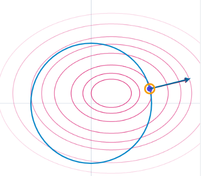
Possible motivation for Lagrange definition of $\mathcal{L}$

Step 1: The Problem, Visualized

Imagine you are a hiker trying to find the highest point on a mountain, but you are forced to stay on a specific trail.

• The Mountain: This is your objective function, $f(x,y)$. The altitude at any point is given by $f$.
• The Trail: This is your constraint, $g(x,y)=c$. It's a specific path on the map.
• Level Curves: The contour lines on a map, where the altitude is constant (e.g., $f(x,y)=1000m$, $f(x,y)=1100m$, etc.).
  You are walking along the trail ($g=c$). When are you at a local maximum or minimum altitude?
  You are at an optimum point when the trail becomes tangent to a contour line of the mountain.
• Why? Think about it: If your trail crosses a contour line, it means you are moving from a lower altitude to a higher one (or vice-versa). If you can still move along the trail and increase your altitude, you're not at the maximum yet!
• The only place where you can't increase or decrease your altitude by moving a tiny step along the trail is the exact point where the trail direction is momentarily parallel to the contour line direction—the point of tangency.

At a constrained optimum, the gradient of the objective function ($\mathrm{\nabla }f$) must be parallel to the gradient of the constraint function ($\mathrm{\nabla }g$).

If two vectors are parallel, one must be a scalar multiple of the other. We'll call that scalar $\lambda$ (lambda).

Step 3: The Stroke of Genius – Creating $\mathcal{L}$

So, at this point, Lagrange knows he has to solve a system of two conditions for a simple 2D problem:

1. $\mathrm{\nabla }f(x,y)=\lambda \mathrm{\nabla }g(x,y)$ (The geometric tangency condition)
2. $g(x,y)=c$ (The original constraint)

The first condition can be rewritten as $\mathrm{\nabla }f(x,y)-\lambda \mathrm{\nabla }g(x,y)=0$. In terms of components, this is:

• $\frac{\partial f}{\partial x}-\lambda \frac{\partial g}{\partial x}=0$
• $\frac{\partial f}{\partial y}-\lambda \frac{\partial g}{\partial y}=0$

And the constraint is:

• $g(x,y)-c=0$

Lagrange's genius was to see that this entire system of equations is exactly what you get if you define a single function and find its unconstrained critical points.

He asked: "What function, if I take its partial derivatives with respect to $x$, $y$, and even $\lambda$, would give me this exact system of equations?"

This leads directly to the definition of the Lagrangian:

2. Coming from Mercury perihelion problem:

Lagrange Multipliers: Constraint Enforcement

When you have constraints like:

1. $g_{ab}{u}^a{u}^b=-1$ (normalization of 4-velocity),
2. ${\mathrm{\nabla }}_a(\rho u^a)=0$ (mass conservation),
   you can impose them in two ways:
3. Restrict the space of fields to only those satisfying the constraints (as you mentioned).
4. Use Lagrange multipliers to dynamically enforce the constraints via the action principle.

We write a Modified Action with Multipliers:

where:

• ${\lambda }_1(x)$, ${\lambda }_2(x)$ are Lagrange multiplier fields (scalar functions over spacetime).
• The original action $\mathcal{E}$ is extended to ${\mathcal{E}}_{\text{new}}$ such that:
  • Varying ${\lambda }_1$ enforces $g_{ab}{u}_{\odot }^a{u}_{\odot }^b=-1$,
  • Varying ${\lambda }_2$ enforces ${\mathrm{\nabla }}_a({\rho }_{\odot }{u}_{\odot }^a)=0$.

Example: Normalization Constraint
For the 4-velocity normalization:

• Add a term ${\int }_M\lambda (g_{ab}{u}^a{u}^b+1){\mathrm{vol}}_g$.
• The variation with respect to $\lambda$ gives back the constraint:

• The variation with respect to $u^a$ now includes $\lambda$:

This modifies the dust equations to dynamically preserve the constraint.