Exterior derivative

See Wikipedia
Coming from differential forms.
It is an antiderivation of degree 1 on the exterior algebra.

1. For a 0-form $df$ is the differential of $f$
2. $d(df)=0$ for 0-forms (for the other differential forms can be deduced)
3. $d(\alpha \wedge \beta )=d\alpha \wedge \beta +(-1{)}^p(\alpha \wedge d\beta )$ where $\alpha$ is a $p$-form.

To make this notion intuitive, we could use the following rough definition:
Definition. Given a $k$-form $\omega$, $d\omega$ is a measure of how dislocated/misaligned are the $(n-k)$-planes represented by $\omega$. For example, in the $(k+1)$-direction provided by the vectors $v_1,\cdots ,v_{k+1}$ we would have:

where $S_{ϵ}$ is a $(k+1)$-plane generated by $v_i$ with volume $ϵ$.
A 1-form in ${\mathbb{R}}^2$ or ${\mathbb{R}}^3$:

Another example: there is no misalignment

A different case: a 1-form in ${\mathbb{R}}^4$. This dislocation/misalignment edges are in this case 2-dimensional spaces (intersection of hyperplanes). The quantity $d\omega (v_1,v_2)$ measures how many misalignments are in that bi-direction.

For visualization of planes, hyperplanes and lines in ${\mathbb{R}}^4$, I made this webpage.

Visualization 1

See xournal 284
Visualize $\omega$ as a family of parallel sheets in each point in space.

The Golden Rule: The lines/tubes of the 2-form $d\omega$ are precisely the edges or vortex lines such that the number of tubes crossing a parallepiped generated by vectors $u,v$ is the same as the net sum of crossing numbers of the path $u+v-u-v$ through the local sheets defined by $\omega$ in nearby points (to guarantee Stokes' theorem).

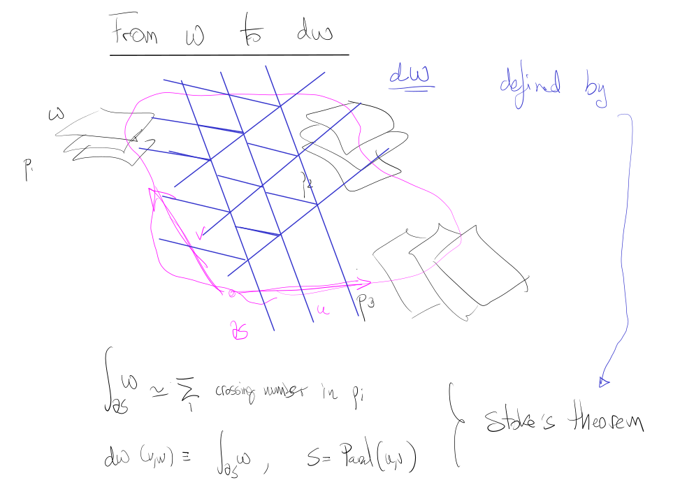
These edges are located where the local sheets of $\omega$ originate, terminate, or twist around one another. In the rest of locations we have kind of parallel sheets, so we cannot have a result different from zero.

We can distinguish three cases:

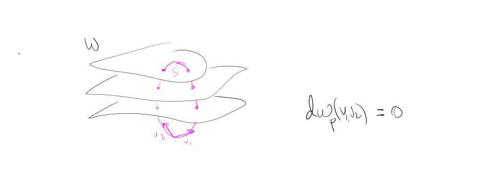
1. Closed 1-form, $d\omega =0$.

We can glue the planes given by $\omega =0$ together.

**2. Frobenius integrable 1-form, $d\omega \wedge \omega =0$

When $\omega \wedge d\omega =0$, the honeycomb structure corresponding to $d\omega$ has walls such that the local sheets $\omega =0$ are linear combination of those walls. So we can "correct" the planes to absorb the edges of the honeycomb structure (with an integrating factor).

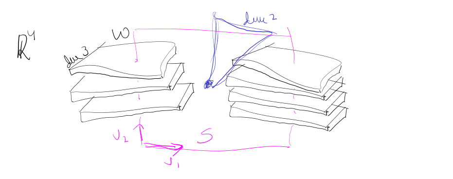
3. Non integrable, $d\omega \wedge \omega \ne 0$

Suppose that when we displace ourselves to the right, the planes $\omega =0$ rotate with axis parallel to the displacement. Then we obtain an emergent honeycomb structure which is by no means parallel to the planes. There is no way to fix this!

1. The "onion" example, $d\omega \wedge \omega =0$

Consider the foliation of spheres

It may be given, instead of by the obvious closed 1-form, by the Frobenius integrable 1-form

The 2-form $d\omega$ corresponds to the lines where the planes hinge.

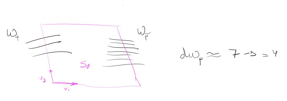
2. The "Extra Pages" Example: $\omega =xdy$

Let's look at a classic non-closed 1-form to see how this works.
The sheets where $\omega =\text{const}$ are planes parallel to the $xz$-plane ($y=\text{const}$). However, notice the coefficient $x$: as you move to the right (increasing $x$), the sheets get packed tighter and tighter together. Their density increases along the $x$-axis.

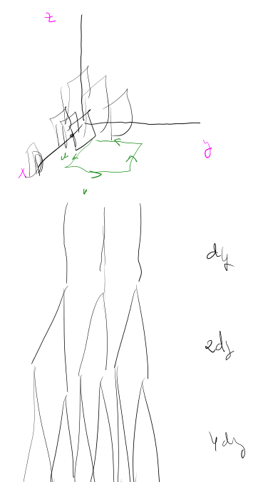
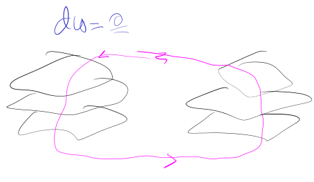
Imagine drawing a square loop in the $xy$-plane from $x=1$ to $x=2$, and $y=0$ to $y=1$. Let's walk around this loop and count how many sheets of $\omega$ we pierce:

• Top and Bottom edges ($dy=0$): We are walking parallel to the sheets, so we pierce 0 sheets.
• Left edge ($x=1$): We walk downward from $y=1$ to $y=0$. Since the density is lower here, let's say we cross 10 sheets in the negative direction.
• Right edge ($x=2$): We walk upward from $y=0$ to $y=1$. Because $x$ is larger, the sheets are twice as dense here! We cross 20 sheets in the positive direction.

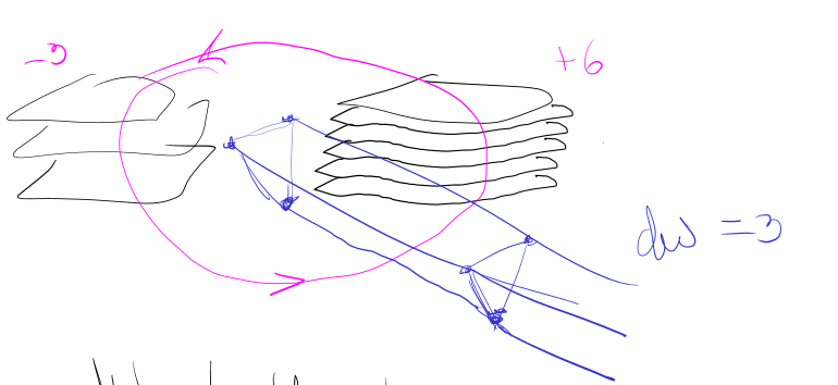
Our net sheets pierced around the loop is $20-10=+10$. If you start at one corner and end up back where you started, how can you have crossed a net total of 10 sheets?
The only logical explanation is that 10 new sheets must have started (originated) inside your square loop. They didn't extend all the way to the left; they popped into existence as the density increased.

Since these extra sheets are 2D surfaces in 3D space, their originating "edges" must be 1D lines. Because the density changes uniformly with $x$, these edges are distributed evenly throughout space, running parallel to the $z$-axis.

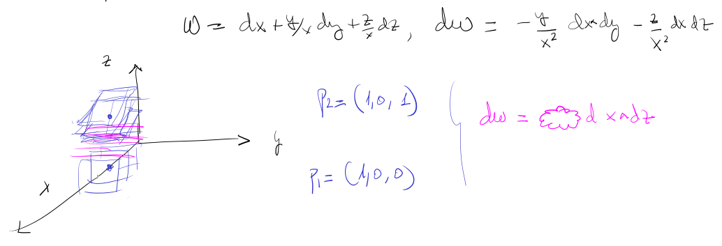
If you calculate the exterior derivative algebraically, you get:

This 2-form represents a uniform grid of lines pointing in the $z$-direction. Each line is exactly one of those "edges" or dislocations where a new sheet of $\omega$ began!

A non integrable example

Consider the contact form $\omega =dy-zdx$ in $(x,y,z)$. This is exactly case 3 (non integrable) above.

See also: visualization of integrability of a Pfaffian system

Visualization 2

See also: visualization of k-forms.

Exterior derivative must be called the negative accumulation meter or production meter.

Case 1: 0-Forms

For a 0-form $f$ (a scalar function), $f$ associate values to points, and $df$ represents the net production of $f$ along a direction:
Example (1D water pipe with a source):
Consider a pipe ($\mathbb{R}$) with water flowing rightward and a point source at $x=3$ injecting 4 units of water per second.

• Let $f(x)$ be the total flow passing point $x$.
  • For $x<3$, $f(x)=0$ (no water yet).
  • For $x\ge 3$, $f(x)=4$ (water added by the source).
• The exterior derivative $df$ is a 1-form encoding the source:$$df=4\delta (x-3)dx,$$

where $\delta (x-3)$ is a Dirac-like concentration at $x=3$.

• Interpretation:
  • $df=0$ where no sources exist (since $f$ is constant).
  • At $x=3$, $df$ spikes to reflect the production of 4 units.
• Integration:

confirming the source’s contribution.

General Intuition:

• $df(X)\approx f(P_2)-f(P_1)$ measures the net change of $f$ along $X=\overrightarrow{P_1{P}_2}$, for $P_1,P_2$ infinitesimally close.
• If $df=0$, $f$ is conserved (no production/loss) along that direction.

Case 2: 1-forms

In the case of a 1-form $\omega$, which associate values to line elements (vectors), exterior derivative tell us how of "something" is being produced in a bivector $u\wedge v$ (a "2-direction"). If we restrict $\omega$ to this area element (with a kind of pullback), the 1-form can be understood like a kind of flow (a 1-form in a 2-dimensional space can be seen as line families at every point, which can be joined together if the 1-form is closed). In this context, $d\omega$ measures how much of this flow is being produced in $u\wedge v$. This is the idea of the infinitesimal Stokes' theorem

In a sense, the value of $d\omega$ in $u\wedge v$ is like measuring how the 1-form varies "along the bivector" $u\wedge v$.

Case 3: 2-forms and more

In the case of 2-forms, for example in ${\mathbb{R}}^3$, these can be visualized as "packages of 1-dimensional fibers" in a neighborhood of each point (in ${\mathbb{R}}^n$, they look like packages of $(n-2)$-dimensional fibers). The value a 2-form assigns to each bivector represents the density of intersections between those fibers and the bivector.

If we apply the exterior derivative of the 2-form to a volume element (a 3-vector), we get something completely analogous to what was described above: pulling back to that "infinitesimally small 3-dimensional space," the 2-form still appears as a kind of one-dimensional flow, and its differential tells us how much is being generated inside (what goes out minus what came in).

If instead of working in ${\mathbb{R}}^3$, we were in ${\mathbb{R}}^n$, the pullback of the 2-form to the 3-vector still appears as a one-dimensional flow—although globally in ${\mathbb{R}}^n$, it may not be.

Why $d^2=0$?

From here it shouldn't be difficult understand why

For 0-forms it is easy: if $\omega =df$, the 2-form $d\omega$ is computed evaluating $\omega$ in sides of the parallelogram $u\wedge v$, which in turn is evaluated in the "vertices". But the latter appear twice in the final computation, but with different sign.
For a 1-form is the same, but a bit more difficult to visualize. In this case $d(d\omega )$ is evaluated in a parallelepiped, and the computation rests, finally, at evaluation on the edges, which appear twice with opposite sign.

The interpretation of $d\omega$ as production (negative accumulation) of a flow in a $k$-vector makes Stokes' theorem trivial. By the way, this interpretation is in some sense given in @needham2021visual page 409.