Visualization of the integrability of a Pfaffian system

Coming from exterior derivative. To summarize, $d\omega$ is a measure of how dislocated/misaligned are the $(n-k)$-planes represented by $\omega$.

The condition $d\mathcal{P}\subseteq \mathcal{P}$ for a completely integrable Pfaffian system can be visualized in the following way:

Case 1: a 1-form in ${\mathbb{R}}^3$

In 3D, you have two possibilities for integrability:
1. Closed 1-form, $d\omega =0$.

We can glue the planes given by $\omega =0$ together.

**2. Frobenius integrable 1-form, $d\omega \wedge \omega =0$

When $\omega \wedge d\omega =0$, the honeycomb structure (recall that it is a 2-form) corresponding to $d\omega$ has walls such that the local sheets $\omega =0$ are linear combination of those walls. So we can "correct" the planes to absorb the edges of the honeycomb structure (with an integrating factor $\mu$). That is you use a single scalar function $\mu$ to separate the sheets of a single 1-form into the differential of a function: $\mu \omega =df$.

Case 2: a pair $⟨{\omega }_1,{\omega }_2⟩$ of 1-forms in ${\mathbb{R}}^3$

It is always integrable, by pure algebra:

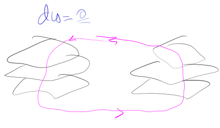
Visually, it works like this:
In case I have two 1-forms, ${\omega }_1,{\omega }_2$, and we can see (both analytically and visually) that

Analytically is not difficult to show that we can find ${\mu }_{ij}$ such that $d({\tilde{\omega }}_i)=d(\sum _j{\mu }_{ij}{\omega }_j)=0$. That is, we can create two combinations of ${\omega }_1,{\omega }_2$ such that they are locally exact.
But we want to see, in the same way that case 1 above, how ${\omega }_1,{\omega }_2$ are distorted to ${\tilde{\omega }}_1,{\tilde{\omega }}_2$ in such a way that $d({\tilde{\omega }}_1)=d({\tilde{\omega }}_2)=0$.
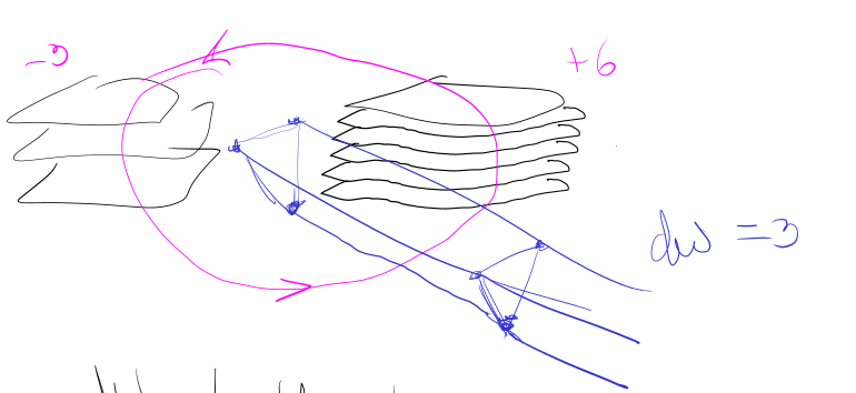
For example, we can imagine that we add ${\omega }_1$ together with a multiple of ${\omega }_2$ to obtain a new 1-form ${\tilde{\omega }}_1={\omega }_1+k{\omega }_2$ whose planes are parallel to the lines $d{\omega }_1$, since the addition of ${\omega }_2$ is kind-of rotating around ${\omega }_1\wedge {\omega }_2$. Even more, we can get $d{\tilde{\omega }}_1$ to correspond to lines parallel to the planes of ${\tilde{\omega }}_1$ with an appropriate choice of the function $k$:

This means that for ${\tilde{\omega }}_1\wedge d{\tilde{\omega }}_1=0$, the 1-form inside the brackets must live entirely in the algebraic span of ${\omega }_1$ and ${\omega }_2$:

This is a Riccati partial differential equation for the shifting function $k$, which always has solution, locally. So by adding $k{\omega }_2$ to ${\omega }_1$ we unroll ${\omega }_1$ to obtain the 1-form ${\tilde{\omega }}_1$ whose dislocation lines are parallel to the planes ${\omega }_1$. Now we can proceed as in Case 1 above. And the same for ${\omega }_2$

Case 3: a pair $⟨{\omega }_1,{\omega }_2⟩$ of 1-forms in ${\mathbb{R}}^4$

In 4D, because we are dealing with a 2-form ideal $⟨{\omega }_1,{\omega }_2⟩$, the scalar integrating factor upgrades to a matrix of integrating factors.
Instead of just rescaling each form individually, we are allowed to mix them together. The algebraic equivalent of absorption here means we can find four smoothly varying functions ${\mu }_{11},{\mu }_{12},{\mu }_{21},{\mu }_{22}$ (forming an invertible matrix) and two independent coordinate functions $f_1$ and $f_2$ such that:

Or, in matrix notation:

What Does This Mean Geometrically?
This matrix transformation completely redefines how we "see" the glued surfaces.

1. From 1-Forms to Exact Coordinates
   By multiplying by this matrix, we have swapped out our rough, twisting, disjointed local 1-forms ${\omega }_1$ and ${\omega }_2$ for two perfect, globally well-behaved functions, $f_1$ and $f_2$.

2. The Intersecting Hyper-sheets
   In 3D, the solution to $df=0$ is a 2D surface ($f=\text{constant}$).
   In 4D:

• $f_1(x,y,z,w)=c_1$ defines a family of perfect 3D hyper-sheets.

• $f_2(x,y,z,w)=c_2$ defines another independent family of perfect 3D hyper-sheets.

3. The Glued 2D Surfaces
   The 2D surfaces you wanted to glue together are the intersections of these two families of hyper-sheets.

At any point in 4D space, the slice where $f_1=c_1$ AND $f_2=c_2$ yields a perfect, smooth 2D surface. Because $f_1$ and $f_2$ are exact derivatives, these 2D surfaces stack together beautifully throughout ${\mathbb{R}}^4$ without a single dislocation or defect line anywhere.

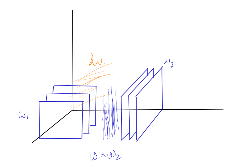
The Visual of "Matrix Absorption"

Think of ${\omega }_1$ and ${\omega }_2$ as two separate, poorly aligned grids of 3D hyper-sheets, both full of dislocation planes (the $d{\omega }_i$ honeycombs) preventing them from passing smoothly through one another.

The diagonal terms of the matrix (${\mu }_{11}$ and ${\mu }_{22}$) act like the 3D integrating factor—they pack and unpack the individual hyper-sheets to match densities. The off-diagonal terms (${\mu }_{12}$ and ${\mu }_{21}$) physically tilt and bend the hyper-sheets of ${\omega }_1$ using the shape of ${\omega }_2$ (and vice versa).

Because the defects are parallel to the distribution ($d{\omega }_i\wedge {\omega }_1\wedge {\omega }_2=0$), this simultaneous packing and tilting perfectly "combs" out all the wrinkles. The two sets of hyper-sheets slip into a flawless, rigid 4D grid, and their 2D intersections line up to form the integrated 2D surfaces.

Would you like to see how this matrix absorption plays out with a concrete algebraic example in 4D, or should we look closer at the geometry of how these 3D hyper-sheets intersect?

Related: For visualization of planes, hyperplanes and lines in ${\mathbb{R}}^4$, I made this webpage.