Laplace transform

Given a complex-valued function $f(t)$ with $t\in \mathbb{R}$, the Laplace transform is a function $F:\mathrm{\Omega }\subseteq \mathbb{C}\to \mathbb{C}$ such that every $F(s)$ represents the weight of the function $e^{st}$ in the decomposition

for any $c$ inside the Region of Convergence (ROC) — the set of $s\in \mathbb{C}$ for which the forward transform converges.

Bilateral vs. unilateral. The formulas above describe the bilateral Laplace transform, where $F(s)={\int }_{-\mathrm{\infty }}^{\mathrm{\infty }}f(t)e^{-st}dt$ and the ROC is a vertical strip ${\sigma }_1<\text{Re}(s)<{\sigma }_2$. The more common unilateral transform integrates from $0$ to $\mathrm{\infty }$, with ROC a right half-plane $\text{Re}(s)>{\sigma }_c$.

A particular case would be the Fourier transform, whose picture corresponds to the case $c=0$ (provided $c=0$ lies in the ROC).

Both transformations have to do with the fact that some spaces of functions are Hilbert spaces, so we have a "basis". The original function can be thought as expressed in the Dirac delta basis, and the Fourier transform and Laplace transform are nothing but the expression of the same function in a different basis. See Fourier, Laplace and Dirichlet relationship.

What basis?, the natural for the generator of the translations.

Why a 1D Line Integral instead of ${\int }_{\mathbb{C}}F(s)e^{st}ds$?

1. Dimensionality: Since $f(t)$ is a 1D function of time ($t\in \mathbb{R}$), it requires a 1D continuum of basis elements to represent it.

2. Linear Independence: Fixing $\text{Re}(s)=c$ yields $s=c+i\omega$, giving a single degree of freedom $\omega \in \mathbb{R}$. The family $\{e^{(c+i\omega )t}{\}}_{\omega \in \mathbb{R}}$ forms an orthogonal basis for $e^{-ct}f(t)$.

3. Overcompleteness: The set of all exponentials $\{e^{st}{\}}_{s\in \mathbb{C}}$ across the entire 2D complex plane is massively redundant (overcomplete). Integrating over all of $\mathbb{C}$ would sum infinitely many duplicate reconstructions of $f(t)$ together, causing the surface integral to diverge.

4. Analyticity: By Cauchy's Integral Theorem, every vertical line $c$ within the ROC carries 100% of the information needed to reconstruct $f(t)$. Shifting $c$ changes the damping factor $e^{-ct}$, but yields the exact same signal.

One Laplace transform or several ones?

It may seems that we have a Laplace transform for each $c$. But we have only one complex variable function $F(s)$, with $s\in \mathbb{C}$. When you calculate the (bilateral) Laplace transform of $f(t)$, $c$ does not exist in the formula:

(The unilateral version integrates from $0$ to $\mathrm{\infty }$ and is often denoted $\mathcal{L}\{f(t)\}(s)={\int }_0^{\mathrm{\infty }}f(t)e^{-st}dt$.)
We can think that since

we have, indeed, different real-valued functions, a 1D restriction of $F(s)$ along the line $\text{Re}(s)=c$:

since

Each "different" Laplace transform is, indeed, a Fourier transform of a "modified" function. And all these 1D slices $F_c(\omega )$ are rigidly bound to one another:

• Identity Theorem: If you know the 1D slice $F_{c_1}(\omega )$ along just one vertical line, you can use analytic continuation to uniquely determine $F_c(\omega )$ along every other valid line $c$ within the ROC.

  • For the bilateral transform (ROC = strip), knowing $F(s)$ on one vertical line determines it everywhere in the strip — but not beyond the boundaries ${\sigma }_1,{\sigma }_2$.
  • For the unilateral transform (ROC = half-plane), the ROC is $\text{Re}(s)>{\sigma }_c$, so analytic continuation extends $F(s)$ to the entire right half-plane — a much stronger statement: one vertical line determines everything.

• None of these 1D slices can vary independently. Once you choose $f(t)$, the entire 2D landscape $F(s)$—and thus all of its 1D slices $F_c(\omega )$ simultaneously—is locked into place.

My interpretation

We can think of Laplace transform $F(s)$ of $f(t)$ as a kind of recipe to construct $f(t)$ from exponential functions $\{e^{st}:s\in \mathbb{C}\}$. But we don't need the whole $F$, we can fix a vertical line in $\mathbb{C}$, $L_c=\{c+i\omega :\omega \in \mathbb{R}\},c\in \mathbb{R}$. Consider the $s$-plane as a collection of all the exponential functions. We can reconstruct $f$ from the exponentials living in any of those lines

Example

This figure illustrates how a single complex landscape $F(s)=\frac{1}{s-i}$ unifies an infinite family of 1D Fourier transforms for the causal signal $f(t)=e^{it}u(t)$. (Here $u(t)$ is the Heaviside step function, for issues of convergence)

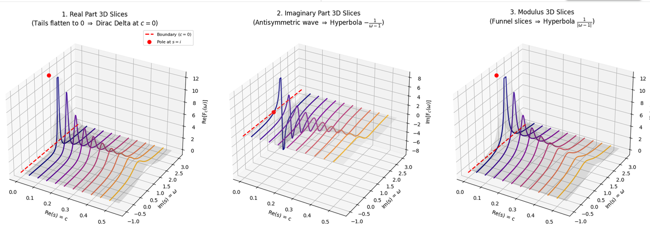
For any vertical line $s=c+i\omega$ within the Region of Convergence ($c>0$), the 1D cross-section $F_c(\omega )$ is literally the continuous Fourier transform of the exponentially damped signal $e^{-ct}f(t)$. As $c$ decreases from $0.50$ down to $0.05$, the damping weakens: the smooth slices of the real part $\text{Re}[F_c(\omega )]$ grow taller (height $1/c$) and narrower while maintaining a constant area of $\pi$. On the boundary $c=0$, the damping vanishes entirely, and this real part collapses into the Dirac delta distribution $\pi \delta (\omega -1)$—matching the real part of the Fourier transform of the causal tone $e^{it}u(t)$. Because all these 1D slices are rigidly bound together across the 2D surface $F(s)$, reconstructing the original signal $f(t)$ via the inverse Laplace transform along any vertical path $L_c$ with $c>0$ yields the exact same underlying function.

Related: non homogeneous linear differential equations using Laplace
Related: Mellin transform.