The Music of Prime Numbers: Rhythms, Laplace Transforms, and the Riemann Zeta Function

Caveat: read together with Riemann hypothesis.

Overview

This note explores the conceptual "music" or "rhythm" of prime numbers. By translating the distribution of primes into a time-domain signal using Dirac delta functions, we can analyze their frequencies using the Laplace Transform. This approach reveals a profound connection between the acoustic/rhythmic properties of prime powers and the non-trivial zeros of the Riemann Zeta Function.

1. The Rhythmic Model of Primes

The foundation of this idea stems from Chebyshev function ( $ψ (x)$ ), which accumulates the logarithm of primes. If we shift this function to a logarithmic scale, $ψ (e^{t})$ , the "jumps" (which occur at prime powers) become evenly spaced for any specific prime.

For the prime $2$ , jumps occur at intervals of $\ln (2)$ .
For the prime $3$ , jumps occur at intervals of $\ln (3)$ .
For the prime $5$ , jumps occur at intervals of $\ln (5)$ , and so on.

Taking the derivative of this function, $\frac{d}{d t} ψ (e^{t})$ , yields a series of "spikes" or Dirac delta functions. Visually and acoustically, these act as a constant metronome or rhythmic beat for each prime.

2. General Mathematical Rhythms

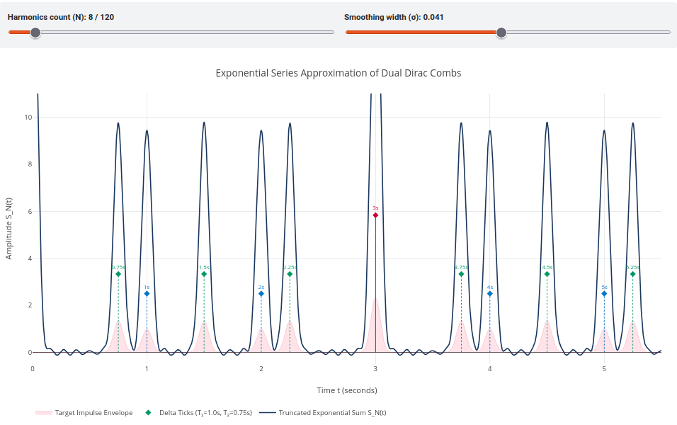
To understand the primes, we first model simple, rational polyrhythms.

Imagine a beat happening every $1$ second and another every $0.75$ seconds. You can play it here. Mathematically, this signal $f (t)$ is a sum of Dirac combs:

f (t) = \sum_{n} δ (t - n) + \sum_{n} δ (t - 0.75 n)

To study the frequencies of this music, we apply the Laplace Transform:

L {f (t)} = \sum_{n} e^{- n s} + \sum_{n} e^{- 0.75 n s}

These are geometric series that evaluate to:

L {f (t)} = \frac{1}{1 - e^{- s}} + \frac{1}{1 - e^{- 0.75 s}}

By finding the poles of this function (where the denominator is zero), we map the specific frequencies that make up the rhythm. Using the Inverse Laplace Transform, summing over these poles perfectly reconstructs the original rhythmic "ticks".
You can explore here how the ticks are located by increasing the number of poles used.
Pasted image 20260925100351.png

3. The Chaotic Polyphony of Primes

Applying this to the prime number spacing, the time-domain signal for the primes is defined by intervals of $\ln (p)$ . It is a polyrhythm made of lots of ticks, ticking at frequencies $\ln (2), \ln (3), \ln (5), \dots$

If we translate this into sound:

A single prime rhythm (e.g., just $2$ ) sounds like a steady metronome.
Combining $2$ and $3$ ( $\ln (2)$ and $\ln (3)$ ) creates an irrational polyrhythm that never repeats.
Adding more primes ( $5, 7, 11 \dots 47$ ) creates a highly chaotic, pseudo-random noise. It lacks any obvious periodicity because the logarithms of prime numbers are linearly independent over the rationals.

The key idea is that we can apply the same technique to this rhythm of the primes!

4. The Truncated Zeta

If we construct the signal using only a finite subset of primes (e.g., just $2$ and $3$ ), the Laplace transform yields an interesting result.

Let's define the function:

\tilde{ζ} (s) = \prod_{p \in {2, 3}} \frac{1}{1 - p^{- s}}

The Laplace transform of our truncated prime signal exactly equals the negative logarithmic derivative of this strange function:

L {f (t)} = - \frac{{\tilde{ζ}}^{'} (s)}{\tilde{ζ} (s)}

To reconstruct the spikes (the rhythms) in the time domain, we need the poles of this expression. The poles of $- \frac{{\tilde{ζ}}^{'} (s)}{\tilde{ζ} (s)}$ correspond to the poles of ${\tilde{ζ}}^{'} (s)$ and the zeros of $\tilde{ζ} (s)$ .
However, $\tilde{ζ} (s)$ has no zeros, and the poles of $- \frac{{\tilde{ζ}}^{'} (s)}{\tilde{ζ} (s)}$ therefore come entirely from the poles of the individual Euler factors:

s = \frac{2 π i k}{\ln p}, p \in {2, 3}, k \in Z .

These are precisely the frequencies of the two periodic pulse trains; summing their residues reconstructs the ticks at $t = k \ln p$ . So far so good.

5. The Riemann Zeta Function

The mathematical magic happens when we stop truncating and include all prime numbers to infinity.

The truncated product becomes the true Riemann Zeta Function:

ζ (s) = \prod_{p} \frac{1}{1 - p^{- s}} = \sum_{n = 1}^{\infty} \frac{1}{n^{s}}

We now apply the Laplace Transform to this "Prime Dirac Comb":

L {\frac{d}{d t} ψ (e^{t})} = \int_{0}^{\infty} (\sum_{p, k} \ln (p) δ (t - k \ln (p))) e^{- s t} d t

Due to the properties of the Dirac delta, the integral simply evaluates $e^{- s t}$ at every spike. Through a standard (but profound) algebraic manipulation involving the Euler Product formula, this infinite sum of primes remarkably collapses into a single analytic expression:

L {\frac{d}{d t} ψ (e^{t})} = - \frac{ζ^{'} (s)}{ζ (s)}

Where $ζ (s)$ is the famous Riemann Zeta function.
That is, the Laplace transform of the prime numbers polyrhythm is exactly the logarithmic derivative of the Riemann Zeta function. Therefore, the "DNA" of the primes is located exactly at the poles of $- \frac{ζ^{'} (s)}{ζ (s)}$ .

Unlike the truncated version, the true Riemann Zeta function does have zeros—specifically, the infinitely many non-trivial zeros lying in the critical strip.

Where do these poles live, and what do they build?

The pole of the Zeta Function ( $s = 1$ ): The pole of $ζ (s)$ at $s = 1$ becomes a pole of $- ζ^{'} (s) / ζ (s)$ with residue $1$ . Its inverse Laplace contribution is $e^{t}$ , the main deterministic trend of the prime-power signal. In the original scale $x = e^{t}$ , this is simply $x$ .
The trivial zeros ( $s = - 2, - 4, - 6, \dots$ ): These zeros become poles of $- ζ^{'} (s) / ζ (s)$ with residue $- 1$ each. In the inverse Laplace transform, they contribute $- \sum_{n = 1}^{\infty} e^{- 2 n t} = - \frac{1}{e^{2 t} - 1}$ , a purely exponentially decaying correction to the prime-power signal.
The non-trivial zeros ( $s = ρ = σ + i ω$ ): Each non-trivial zero becomes a pole of $- ζ^{'} (s) / ζ (s)$ at $ρ$ and contributes $- e^{ρ t}$ to the prime-power signal. The zero sum is understood symmetrically; conjugate pairs produce the oscillations, while $σ$ determines the envelope.

Together, these three components give the following analytical expression for the prime-number polyrhythm:

\frac{d}{d t} ψ (e^{t}) = e^{t} - \frac{1}{e^{2 t} - 1} - \sum_{ρ} e^{ρ t}

You can explore here how the primes are located by increasing the number of non-trivial Riemann zeta zeroes are used!
Pasted image 20260925105851.png
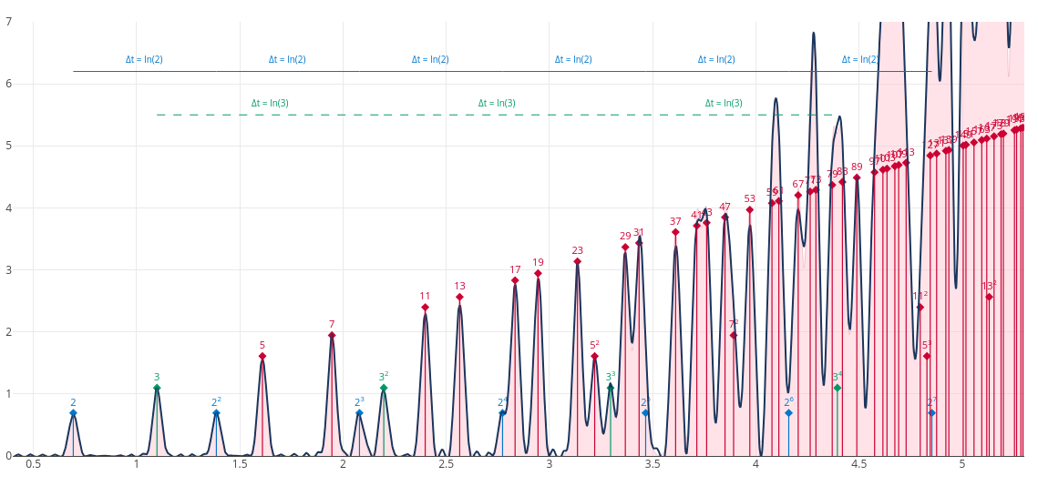
So the zeros of the Riemann zeta function encode the information about primes. Now, you can proceed to understand the importance of Riemann hypothesis.